“Obscured by Clouds” - don’t let portfolio design be obscured by market timing

Introduction

While the title of this piece refers to a famous Pink Floyd album, the theme of the title and the timing of the release, in June 1972, point directly to the two key ideas raised in the enclosed article, as follows:

• First, we would like to explore the idea of obfuscation; the obfuscation of inflation linked bond (ILB) returns by mark-to-market volatility
• Second, we would like to highlight what happened in the late nineteen sixties, and nineteen seventies, and what essential role ILBs play in such high inflationary environments

By analysing a longer period, we include inflation risks, which are not apparent in shorter term studies. Accordingly, we simulate ILB returns since 1962, and compare and contrast these results in several ways, so as to focus attention on portfolio design, and away from issues of market timing. Specifically, we explore the portfolio design with ILBs in the following four ways:

1. Provide details of our long term ILB simulation.
2. Consider the main argument for owning ILBs; the direct insurance against inflation.
3. Consider how secondary market pricing obscures the argument for owning ILBs.
4. Bearing sections 2 and 3 in mind, we then focus attention on the portfolio design benefits of ILBs.

1          Simulation details

While we have limited data on ILB yields, we do have extensive daily data on nominal yields, and we can simulate the ILB performance using the following two assumptions, where we break ILB returns into the following two components:

• Rolling yield above inflation: here, we assume a modest 2% above the prevailing rate of inflation. For explanatory purposes, we can refer to this aspect of ILB return as “R”, and
• Capital gain/loss: since ILB prices generally move about one third of the movement of nominal (fixed rate bond), we can use one third of the capital changes in the nominal bonds as a measure for changes in the ILB. For explanatory purposes, we can refer to this aspect of ILB return as “K”. This ratio is roughly the average accepted ratio of movement within bond markets, although the ratio can change dramatically from period to period.

This approach is adopted for the period from 2 January 1962 to 4 August 1998. After that date, until 20 September 2013, we use actual ILB yields to estimate both capital changes, and rolling yield above inflation. Daily returns are then summed on a rolling 250 trading day basis, so as to derive annual return estimates, for the entire simulation period.

Now, this disaggregation of ILB return, into “R” and “K”, really helps in terms of understanding the role of ILBs in a portfolio, as discussed in section 2 and 3 below.

2          Link to inflation, or “R”

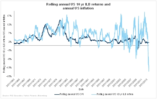
One of the most important aspects of ILBs is the way the security provides a direct linkage to the CPI, and no other security offers this linkage; all other linkages are implied and are not reliable in any time frame. Despite the claims to the contrary, there is a large amount of evidence to support the fact that equities do not provide a hedge against inflation, as we have noted many times. In particular, given our assumptions of a 2% over inflation rolling return, in the early part of our simulation, we can see in Figure 1 how beneficial that rolling return was when inflation rose; in the late nineteen sixties and seventies; around the time that our Pink Floyd album, “Obscured by Clouds”, was released.

It is this characteristic of return, or “R”, as we refer to it in our simulation, that investors need to focus on, as this return stream is not offered by nominal fixed rate bonds, which pay a fixed coupon and redemption payment. Fixed rates do not vary with inflation, while ILBs are designed to do just that; very handy in a situation where inflation is rising.

Figure 1

3.         Capital price changes or “K”

Now that one has seen how part of the ILB return, which we term “R” varies with inflation, the problem we now face is how the changes in secondary market pricing impact total returns. These variations can be large and obscure why ILBs should be in a portfolio. Since financial markets do not have perfect knowledge, they make guesses about what real interest rates and inflation will be in the future. However, that is all they are, and one guess is followed by the next guess; all are incorrect in the absence of perfect foresight. When we obtain perfect foresight, then we will not need a secondary market for ILBs, but until then, we need to recognise capital price changes for what they are; a series of mistaken guesses on the forward trajectory of real yields.

A recent example might be helpful in getting this idea across, as illustrated in Figure 2 below, as follows:

• 12 months ago, financial markets were pricing in perpetual low growth and US ILB yields were very low, around negative 83 basis points. This meant that investors bought 10 year ILBs and were happy to receive inflation, or around 2% less 83 basis points (117bps). Such an expectation drove up ILB secondary market prices to a point where the annual return on 10 year ILBs had never been higher, around January 2012.
• Then, markets substituted the expectation, or guess, as generated in early 2012, with another guess. Now, the markets expected that inflation would rise along with growth. This guess was then magnified by talk a reduction in quantitative easing (QE), or a “taper” of QE. This then sent the annual return on ILBs to an all-time current low
• Both of these guesses remain incorrect, as no one knows the forward trajectory of inflation with any certainty, and the two annual returns effectively cancel each other out.

Figure 2

Notice how changes in “K”, as embedded in the total annual returns of ILBs, and as shown by the light blue line in Figure 2 above, effectively obscure the relationship that was illustrated in Figure 1. While, in Figure 1 “R” was seen to move up and down with inflation, as shown by the dark blue line in Figure 2 above, one cannot see that relationship in Figure 2 because total return effectively obscures the observation found in Figure 1. Specifically, the light blue line represents the addition of “R” with “K”.

In the case of Australian credit ILBs (which have been impacted by the recent moves in US Treasury ILBs) in part the rise in yields has been the demise of bond insurance companies, while most of the rise has been the result of a change in the institutional market, where mandate changes have forced sales. All these changes just make the Australian credit ILB the cheapest ILB market in the developed world. Countries like the UK and South Africa have some credit ILBs, yet the yields on offer are not attractive; nowhere near what Australian investors enjoy.

4          Portfolio design

Section 3 tells us is that we should try to focus on the relationship between inflation and ILBs, as shown in Figure 1 and driven by “R”, as opposed to the distorting influences of “K”, as shown in Figure 2. In other words, try and focus on the design of the portfolio, and not the timing issues. If, you have an adequate allocation to ILBs, then you should take advantage of abnormal movements in secondary market pricing, yet most portfolios do not have anywhere near what they need in terms of allocation to ILBs. Again, the main reason investors do not have enough ILBs, is that investors are effectively being “obscured by the clouds” of market price changes; by looking at Figure 2 and “K” too much and Figure 1, and “R”, not enough.

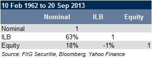
In addition, because of the special feature in ILBs, what we term “R”, ILBs are not perfectly correlated to nominal bonds, and have different correlations to equities, when compared to nominal bonds, as shown in Table 1, which shows the correlation between annual returns with more than 13,000 annual return observations. Correlation measures the degree to which two variables move together, where low correlation means two variables do not move together, and high correlation, towards 100%, means that two variables move together.

Table 1: Source: FIIG Securities, Bloomberg, Yahoo Finance

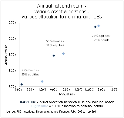
This correlation analysis means that adding ILBs to the fixed income section of the portfolio can reduce risk, while not reducing return, as shown in Figure 3 below. Notice that the larger the bond allocation, which we recommend as part of the way to address sequence risk, the bigger the benefits of ILBs, in terms of risk reduction. While the dark blue dot allocates the fixed income allocation equally between 10 year US government ILBs and 10 year US government nominal bonds, the light blue only allocates to nominal bonds.

Figure 3

Conclusion

The main reason for holding ILBs in a portfolio is to insure against inflation, especially the type of high inflation witnessed in the nineteen seventies. Secondary market pricing swings can, and often do, obscure this important fact. Hence, in this article, we show how ILBs help reduce the risk of inflation, as well as portfolio risk; the greater the allocation, the bigger the benefit of ILBs. As you listened to the “Obscured by Clouds” album in 1972, you would have been much more content having a meaningful allocation to ILBs in your investment portfolio, when compared to either nominal bonds or equities. Capturing what we term “R” is what ILBs are all about, and it remains as relevant today as it was in 1972.

Also, what happens to US treasuries impacts markets like the Australian market; higher US treasury ILB yields have pushed up AUD ILB yields. While our credit ILBs have been cheap, this recent move makes them even better value, to the point where local investors have the opportunity to purchase high credit quality ILBs at real yields that are just not available in the rest of the developed world. However, these considerations about market timing are again secondary to the primary portfolio design questions considered herein. It is portfolio design, as primarily expressed by “R” and not market timing, as expressed by “K” which should remain your top priority.