Sequencing risk - Part 2

After more than 20 years without a recession in Australia, the typical Australian investor has become complacent about risk, and become one of the most aggressive investors in the OECD. All this is fine, until another recession hits. Importantly, it is not an “if” but a “when”, and sequencing risk helps you think about the impact of timing of risk on the portfolio; of what might happen when the next recession strikes.

“Growth” comes with a price, and that price is measured in variety of ways. Sequencing risk is one way we analyse the timing of portfolio performance, where the differences in return sequence can lead to very large differences in portfolio accumulated values, at any point in the investment cycle either before or after retirement. This week we make the analysis a little more practical than last week, as we now consider some longer term US data on a theoretical portfolio of 75% equities, using data on the S&P 500, and 25% 10 year corporate bonds, using the US ten year fixed swap rate plus 100 basis points. Initially, we present the original and reverse sequence of returns, and then we look at how these sequences can severely impact the accumulated value of investments, over time. We are not alone in highlighting this form of risk, as recent work of Dr. Ken Henry, former head of the Australian Treasury and Chairperson of the “Australia’s Future Tax System Review”, otherwise known as the Henry Review into Taxation, shows. Importantly, the differences in accumulated value, between the two sequences is “not immaterial”, as we saw Dr. Henry describe them in Part 1 last week.

In this article we detail:

1. Some longer dated return sequence data from the US.
2. An analysis of how this return sequence impacts the accumulated portfolio return over time.
3. Some of the commentary from Ken Henry on the subject of sequencing risk.

 1.         Return sequences

Using very long term US equity and bond performance data from 1964 we can show the significant variations in the yearly data (not the accumulated value of the portfolio) with regard to the two opposite return sequences. For example, consider Figure 1 below, where we show portfolio returns for a 75% equity portfolio and 25% 10 year bond portfolio, which begins with $100,000, and has regular $30,000 contributions at the start of each calendar year. Here, the dark blue line shows the original sequence, while the light blue line shows the exact opposite sequence; only one of a variety of possible return sequences. Notice the large difference between these returns especially in the early period, around 1974 to 1984, where the light blue line, or the opposite sequence, is consistently above the dark blue line, or the original sequence.

Figure 1

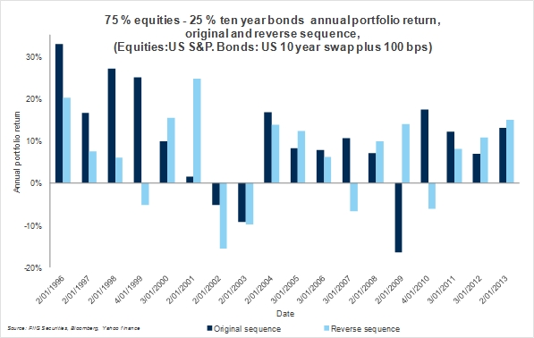
Figure 2 provides a little more focus on more recent data from 1996 to 2013, where we see some very large variations in portfolio return, just by comparing the original sequence with the reverse sequence. Notice, the key return years like 2001, where the original sequence returns are poor, while they are great with the reverse sequence( in 2009) where the original sequence is very disappointing, but the opposite is the case with the reverse sequence.

Figure 2

2          Impact of return sequence on accumulated portfolio value

We have now established that variations in portfolio returns can be very large, just by reversing the sequence of returns. Next, we look at the impact of these large variations on the accumulated value of a portfolio that starts with a $100,000 investment and has $30,000 contributions at the start of each calendar year for 50 years.

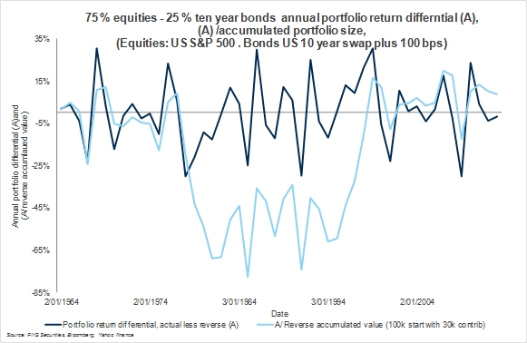
In Figure 3, we show the yearly portfolio return differentials as the dark blue line, and the accumulated impact of those differentials as the light blue line. As we mentioned above, the difference between the two sequences is very large in the 1974-1984 period, and the impact on the accumulated portfolio value is substantial. As Figure 3 shows that differential peaks at almost 85% of the reverse sequence accumulated value size. Hence, around 1984 the value of the portfolio, which was accumulating in the same way as the original sequence, was 80% less than the value of the original sequence, when you express that differential as a percentage of the accumulated value of the reverse sequence. From then, however, the reverse sequence tends to catch up with the original sequence.

Figure 3

While the accumulated differential is large, during the middle of the analysis period, this analysis indicates that exposing your portfolio to the volatility of equity risk opens up the prospect of significant variations in the accumulated value of your portfolio. If you get the timing right sequencing risk may not be a problem.

Then again, you may not “get it right”, and the sequencing risk can easily devastate your retirement nest egg.

Henry

Portfolio volatility is a risk that needs to be minimised, particularly as you get closer to retirement and you don’t have time to recoup losses. A downturn in the economy and thus the price of growth assets can hit the portfolio at the wrong time. It is always the wrong time to incur a loss, yet as investors’ age, the ability to recover from large loss falls, as the effective investment horizon shortens. So, while sequencing risk is omnipresent, being applicable to both the accumulation and de-cumulation phase of saving, the issue of sequencing risk gradually rises in importance as the investment time horizon becomes less and less. What many financial planners and advisors do, when confronted with a client that has not enough savings to fund an increasingly long retirement, is to “go for growth”; where “growth” assets effectively solve the problem and increase savings to the level required for longer retirement periods. We think this is entirely the wrong approach, and we have support from Ken Henry, as noted below

The idea that longevity risk is best managed by increasing one’s exposure to equities, and thereby taking on a greater degree of sequencing risk, is even more worrying [than the idea that one needs to take on more risk with higher life expectancy]. It is certainty better than encouraging an aged pensioner to put her pension cheque through a poker machine – since the expected gain in the former case is positive, while in the latter case is clearly negative – but the actual outcome can be just as disappointing ... I know it’s an old-fashioned notion, but I do think risks, and that includes sequence risk, are managed best by taking out insurance, not by substituting one set of risks for another [brackets added] (“Why is portfolio allocation to domestic fixed income low in Australia and should it be increased?”, Address to the 11^th Australian Securitisation Forum Conference, 23 October 2012, Hilton Hotel, Sydney, p.5).

In the next article in the series, we explore the ways in which investors can reduce portfolio volatility, using bonds, thus reducing the impact of sequencing risk on the investment portfolio.

Conclusion

Retiring on 50% less than you planned is not a prospect that most retirees want to think about. Yet, if you have too much volatility in your investment portfolio, then you are effectively saying that you accept such a scenario. In many ways, the global financial crisis may just be a preview of portfolio return, and that means you need to be conservative. We already know that the consumer has become conservative, as the RBA have reminded us recently, and we would argue that the time is now right for the investor to become conservative; to take sequencing risk as seriously as former significant government officials, like Ken Henry, do. While the return sequence differential can be extreme, the impact on the portfolio’s accumulated value can be devastating. Cutting underlying portfolio volatility helps manage sequencing risk.  Bonds are low risk and have more consistent returns so help stabilise overall portfolio return and lower sequencing risk.